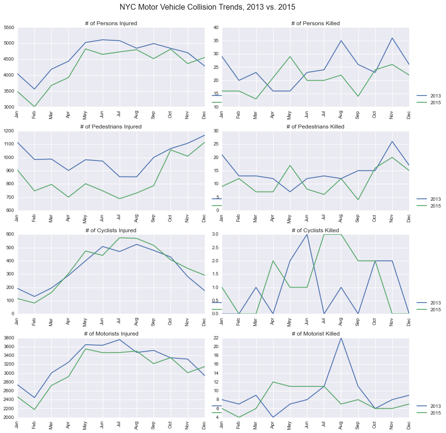
What months are most dangerous for pedestrians and cyclists?

Exploring the NYPD Motor Vehicle Collision open data set using python.

Python has become a popular programming language for data analysis. It is free, flexible, easy to learn and has a robust ecosystem of useful tools. The following tutorial will run some basic wrangling and analysis tasks using Python and a few of it’s data-oriented tools. We will look at NYC Motor Vehicle Collision data set provided by the New York Police Department via NYC Open Data.

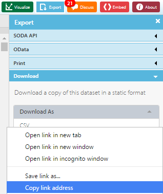
Identifying the data source

Click ‘Export’ and then copy the link address of the CSV file. fig1

Set up the environment

import matplotlib.pyplot as plt
import matplotlib.dates as mdates
import numpy as np
import os
import pandas as pd
import seaborn as sns
%matplotlib inline

Load the raw data

Pandas has an object called a ‘DataFrame’, which is similar to a spreadsheet tab or a SQL table. DataFrames are great for working with clean, tabular data containing rows and columns. Load the CSV into a pandas DataFrame object.

url = 'https://data.cityofnewyork.us/api/views/h9gi-nx95/rows.csv?accessType=DOWNLOAD' # Date of download = 5/8/2016
df = pd.read_csv(url)
df.head()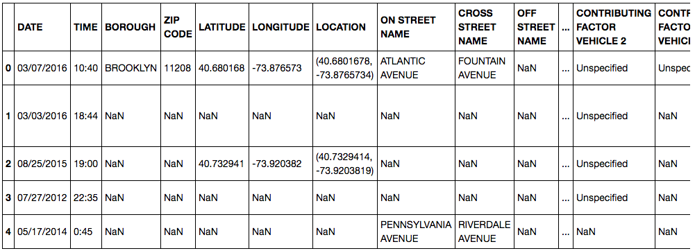

fig1

Clean the data

Combine DATE and TIME columns into one column and convert to datetime format for timeseries analysis

data['Date'] = df['DATE'] + ' ' + df['TIME']
data['Date'] = pd.to_datetime(data['Date'], format='%m/%d/%Y %H:%M')

Bring in other relevant columns as they are (with nicer column headings)

data['Borough'] = df['BOROUGH']
data['On Street'] = df['ON STREET NAME']
data['Cross Street'] = df['CROSS STREET NAME']
data['Persons Injured'] = df['NUMBER OF PERSONS INJURED']
data['Persons Killed'] = df['NUMBER OF PERSONS KILLED']
data['Pedestrians Injured'] = df['NUMBER OF PEDESTRIANS INJURED']
data['Pedestrians Killed'] = df['NUMBER OF PEDESTRIANS KILLED']
data['Cyclists Injured'] = df['NUMBER OF CYCLIST INJURED']
data['Cyclists Killed'] = df['NUMBER OF CYCLIST KILLED']
data['Motorist Injured'] = df['NUMBER OF MOTORIST INJURED']
data['Motorist Killed'] = df['NUMBER OF MOTORIST KILLED']
data['Contributing Factor Vehicle 1'] = df['CONTRIBUTING FACTOR VEHICLE 1']
data['Contributing Factor Vehicle 2'] = df['CONTRIBUTING FACTOR VEHICLE 2']
data['Contributing Factor Vehicle 3'] = df['CONTRIBUTING FACTOR VEHICLE 3']
data['Contributing Factor Vehicle 4'] = df['CONTRIBUTING FACTOR VEHICLE 4']
data['Contributing Factor Vehicle 5'] = df['CONTRIBUTING FACTOR VEHICLE 5']
data['Unique Key'] = df['UNIQUE KEY']
data['Vehicle 1 Type'] = df['VEHICLE TYPE CODE 1']
data['Vehicle 2 Type'] = df['VEHICLE TYPE CODE 2']
data['Vehicle 3 Type'] = df['VEHICLE TYPE CODE 3']
data['Vehicle 4 Type'] = df['VEHICLE TYPE CODE 4']
data['Vehicle 5 Type'] = df['VEHICLE TYPE CODE 5']

Sort by data and reset index

data.sort('Date', ascending=True, inplace=True)
data.reset_index(drop=True, inplace=True)

Convert categorial columns to category dtype

data['Unique Key'] = data['Unique Key'].astype('string')
data['Contributing Factor Vehicle 1'] = data['Contributing Factor Vehicle 1'].astype('category')
data['Contributing Factor Vehicle 2'] = data['Contributing Factor Vehicle 2'].astype('category')
data['Contributing Factor Vehicle 3'] = data['Contributing Factor Vehicle 3'].astype('category')
data['Contributing Factor Vehicle 4'] = data['Contributing Factor Vehicle 4'].astype('category')
data['Contributing Factor Vehicle 5'] = data['Contributing Factor Vehicle 5'].astype('category')
data['Vehicle 1 Type'] = data['Vehicle 1 Type'].astype('category')
data['Vehicle 2 Type'] = data['Vehicle 2 Type'].astype('category')
data['Vehicle 3 Type'] = data['Vehicle 3 Type'].astype('category')
data['Vehicle 4 Type'] = data['Vehicle 4 Type'].astype('category')
data['Vehicle 5 Type'] = data['Vehicle 5 Type'].astype('category')

data.head()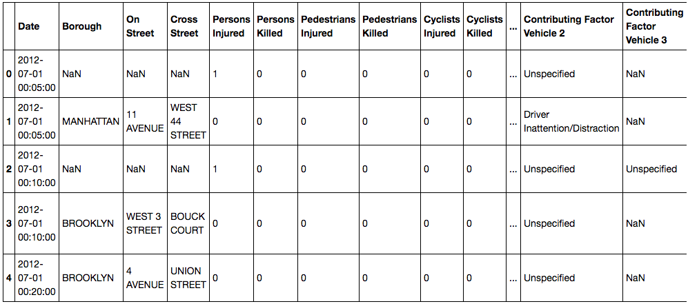

fig

Exploratory data analysis

Calculte the total deaths and injuries per month

per = data.Date.dt.to_period("M")
g = data.groupby(per)
g.sum()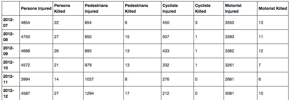

fig

# Make separate dataframes per year
data2013 = data[(data['Date'] >= '2013-01-01') & (data['Date'] <= '2014-01-01')]
data2014 = data[(data['Date'] >= '2014-01-01') & (data['Date'] <= '2015-01-01')]
data2015 = data[(data['Date'] >= '2015-01-01') & (data['Date'] <= '2016-01-01')]
data2016 = data[(data['Date'] >= '2016-01-01') & (data['Date'] <= '2017-01-01')]


# Group each year by month
per2013 = data2013.Date.dt.to_period("M")
per2014 = data2014.Date.dt.to_period("M")
per2015 = data2015.Date.dt.to_period("M")
per2016 = data2016.Date.dt.to_period("M")

g2013 = data2013.groupby(per2013).sum()
g2014 = data2014.groupby(per2014).sum()
g2015 = data2015.groupby(per2015).sum()
g2016 = data2016.groupby(per2016).sum()

g2015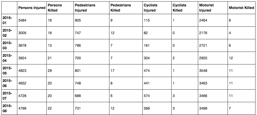

fig

Plot motor vehicle collision injuries and deather by type, over time

fig, ax = plt.subplots(nrows=4, ncols=2, figsize=(12,12))

# Plot persons injured per Month by Year
ax[0,0].plot(g2013['Persons Injured'], label='2013')
#ax[0,0].plot(g2014['Persons Injured'], label='2014')
ax[0,0].plot(g2015['Persons Injured'], label='2015')
ax[0,0].set_title('# of Persons Injured')
ax[0,0].set_xlim(0,11)

# Plot persons killed per month by year
ax[0,1].plot(g2013['Persons Killed'], label='2013')
#ax[0,1].plot(g2014['Persons Killed'], label='2014')
ax[0,1].plot(g2015['Persons Killed'], label='2015')
ax[0,1].set_title('# of Persons Killed')
ax[0,1].set_xlim(0,11)
#ax[0,1].set_ylim(0,40)

# Plot pedestrians injured per month by year
ax[1,0].plot(g2013['Pedestrians Injured'], label='2013')
#ax[1,0].plot(g2014['Pedestrians Injured'], label='2014')
ax[1,0].plot(g2015['Pedestrians Injured'], label='2015')
ax[1,0].set_title('# of Pedestrians Injured')
ax[1,0].set_xlim(0,11)

# Plot pedestrians killed per month by year
ax[1,1].plot(g2013['Pedestrians Killed'], label='2013')
#ax[1,1].plot(g2014['Pedestrians Killed'], label='2014')
ax[1,1].plot(g2015['Pedestrians Killed'], label='2015')
ax[1,1].set_title('# of Pedestrians Killed')
ax[1,1].set_xlim(0,11)
#ax[1,1].set_ylim(0,40)

# Plot cyclists injured per month by year
ax[2,0].plot(g2013['Cyclists Injured'], label='2013')
#ax[2,0].plot(g2014['Cyclists Injured'], label='2014')
ax[2,0].plot(g2015['Cyclists Injured'], label='2015')
ax[2,0].set_title('# of Cyclists Injured')
ax[2,0].set_xlim(0,11)

# Plot cyclists killed per month by year
ax[2,1].plot(g2013['Cyclists Killed'], label='2013')
#ax[2,1].plot(g2014['Cyclists Killed'], label='2014')
ax[2,1].plot(g2015['Cyclists Killed'], label='2015')
ax[2,1].set_title('# of Cyclists Killed')
ax[2,1].set_xlim(0,11)
#ax[2,1].set_ylim(0,40)

# Plot motorists injured per month by year
ax[3,0].plot(g2013['Motorist Injured'], label='2013')
#ax[3,0].plot(g2014['Motorist Injured'], label='2014')
ax[3,0].plot(g2015['Motorist Injured'], label='2015')
ax[3,0].set_title('# of Motorists Injured')
ax[3,0].set_xlim(0,11)

# Plot motorists killed per month by year
ax[3,1].plot(g2013['Motorist Killed'], label='2013')
#ax[3,1].plot(g2014['Motorist Killed'], label='2014')
ax[3,1].plot(g2015['Motorist Killed'], label='2015')
ax[3,1].set_title('# of Motorist Killed')
ax[3,1].set_xlim(0,11)
#ax[3,1].set_ylim(0,40)

# Add months as x-axis ticks
months = ['Jan', 'Feb', 'Mar', 'Apr', 'May', 'Jun', 'Jul', 'Aug', 
          'Sep', 'Oct', 'Nov', 'Dec']
plt.setp(ax,xticks=range(len(months)), xticklabels=months)

# Add main title
plt.suptitle('NYC Motor Vehicle Collision Trends, 2013 vs. 2015', fontsize=16, y=1.03)

# Rotate x-ticks to vertical
for ax in fig.axes:
    plt.sca(ax)
    plt.xticks(rotation=90)
    i = 0
    if i%2 == 0:
        ax.legend(bbox_to_anchor=(1.03, 0), loc='lower left', borderaxespad=0.)
    i=i+1

fig.tight_layout();

fig